C1 · INVERTER DYNAMICS · CORE COURSE
IBR Dynamic
Modeling &
Simulation
Start with the circuit.
Explain the response.
Make an informed decision.
A complete learning sequence: why a model is needed, how its structure produces the equations, and what its response can establish.
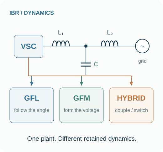
Physical structure → synchronization → system behavior
THE THREAD THROUGH THE COURSE
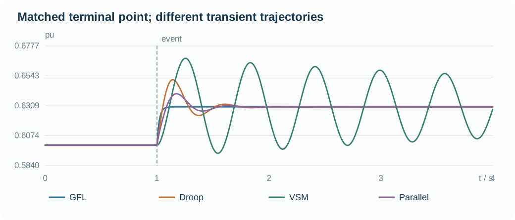
One interconnection target.
Why different responses?
A 10 kVA, 400 V, 50 Hz project compares GFL, droop, VSM and parallel hybrid realizations. The team matches initial PoC power to P = 0.6 pu, Q = 0, then applies a +0.03 pu power command.
Work backward from this decision: establish boundaries and coordinates, understand electrical storage and synchronization, then distinguish model mechanisms from operating-point and numerical effects.
THREE STAGES, ONE COHERENT ARGUMENT
The learning path
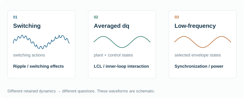
What must the model retain?
Establish the physical foundation
Boundaries, coordinates and stored energy make the equations interpretable.
C1-01 60 min
System Boundaries and Model Representations
Which model is sufficient for the decision?
Open lesson →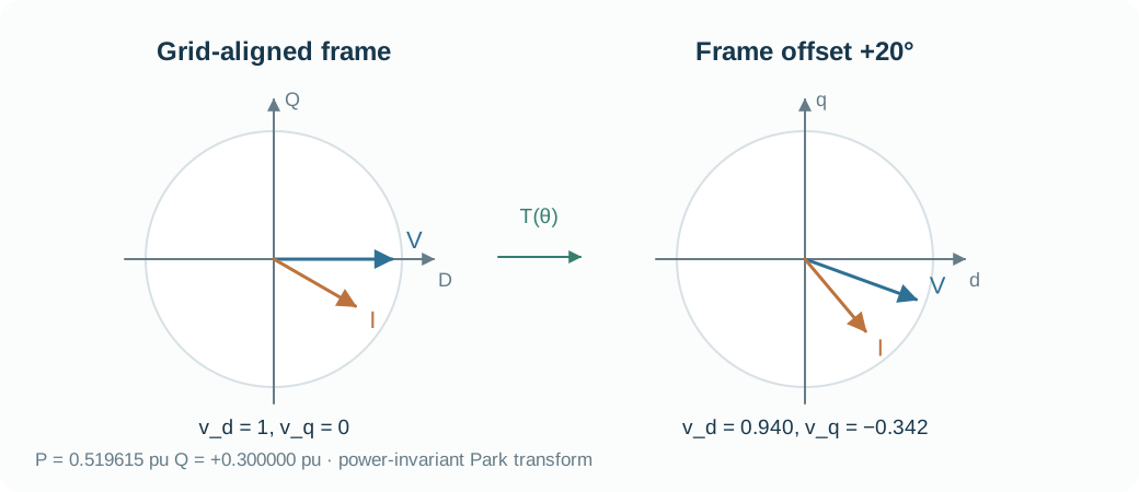
C1-02 60 min
Reference Frames and Per-Unit Conventions
How can rotating coordinates preserve the same physics?
Open lesson →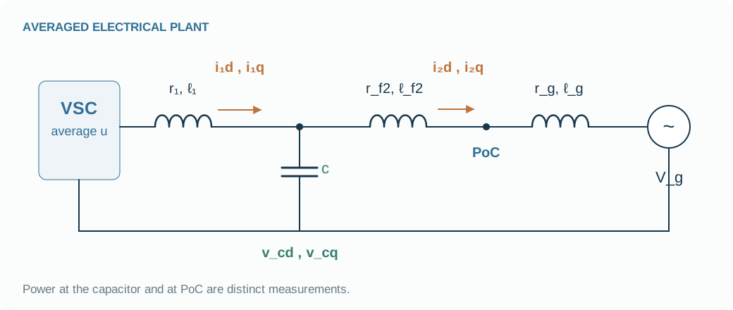
C1-03 60 min
Averaged Converter and LCL Plant
Where does an electrical oscillation come from?
Open lesson →Where does the angle come from?
Understand the synchronization mechanism
Follow an acquired angle, generate one through droop, then add speed dynamics.
C1-04 90 min
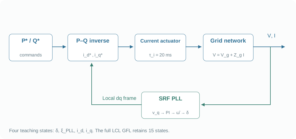
PLL and Grid-Following Control
When the grid angle moves, what does GFL follow?
Open lesson →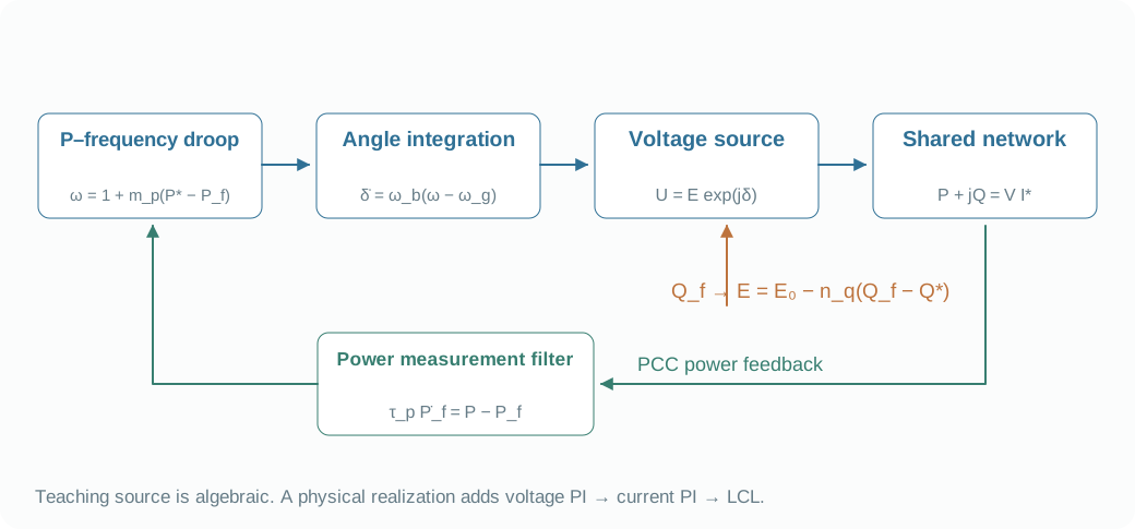
C1-05 90 min
Droop Grid-Forming Control
How does a power mismatch create a voltage angle?
Open lesson →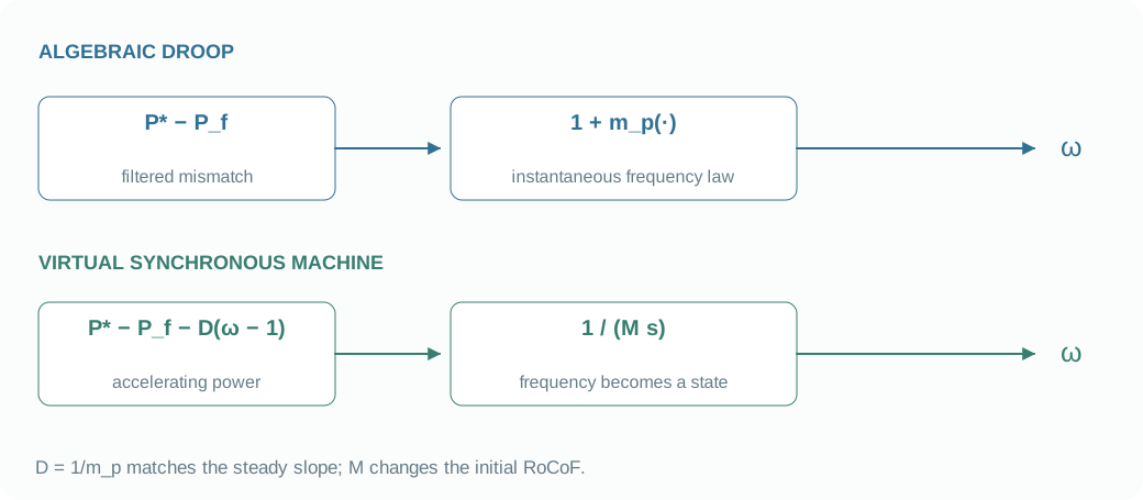
What evidence supports the decision?
Make a defensible engineering judgment
Connect branches, design transitions and compare models on common terms.
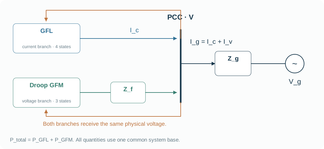
C1-07 90 min
Parallel GFL–GFM Hybrid Models
Why is a shared PCC more than two separate simulations?
Open lesson →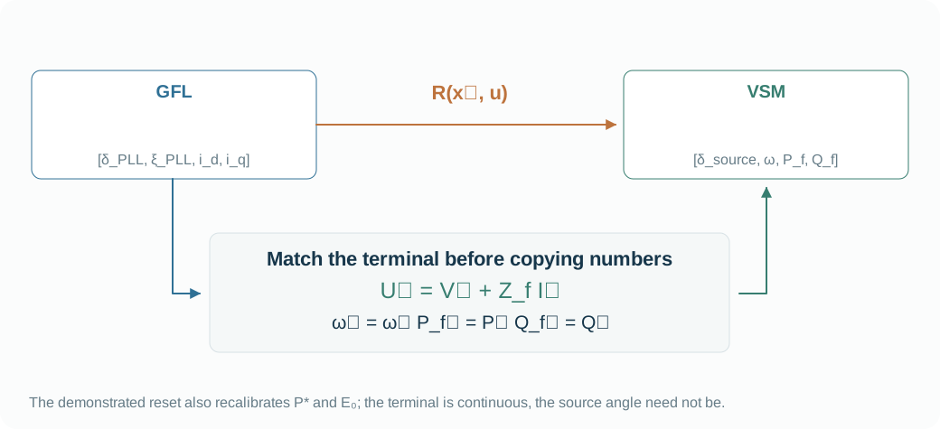
C1-08 90 min
Mode-Switching Hybrid Models
What must remain continuous when the controller changes?
Open lesson →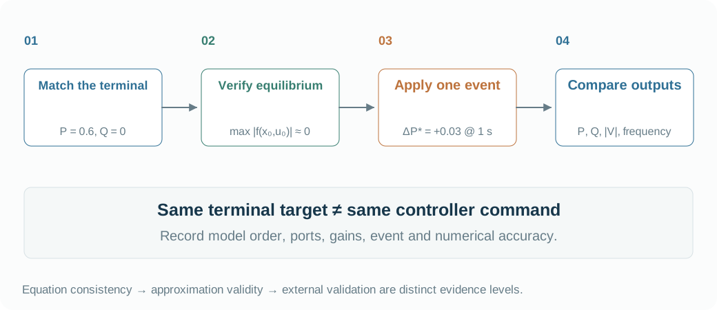
C1-09 90 min
Equilibrium, Disturbances, and Fair Comparison
What evidence makes a model comparison credible?
Open lesson →HOW EACH LESSON WORKS
Make a prediction.
Let the experiment answer.
Basic circuits, differential equations, and introductory Python.
- A case poses the questionSet the engineering context and the decision.
- Diagrams connect the derivationConnect structure, states, feedback and equations.
- A worked case builds a predictionCalculate direction and scale before plotting.
- The lab tests the judgmentChange parameters, explain responses and inspect scope.
CAPSTONE · A REPRODUCIBLE DECISION BRIEF
From different curves to an explanation you can defend.
Write a two-page model-selection brief for a specific interconnection study. Match ports and operating points, compare at least two disturbances, attach an executable experiment and qualify the evidence.
Take the course with you
The notebook includes diagrams, derivations, cases and the complete standard-library solver.
Teaching levels and model scope
Lesson 2 checks the power-invariant transform; Lesson 3 retains the six-state averaged LCL; Lessons 4–9 use nominal-frequency algebraic networks and ideal actuators to isolate synchronization and hybrid interfaces. These independent teaching realizations are separate from the source full-order controllers and official REGFM_C1 implementation. Residuals establish equation consistency; higher-order comparison and external validation require further work.