LESSON 05 / 09 · MODELING & SIMULATION
Droop Grid-Forming Control
How does a power mismatch create a voltage angle?
THE CASE
How does a power mismatch create a voltage angle?
The operator raises P* by 0.03 pu. A GFM source cannot assign terminal power directly: it must change frequency, move its angle and let the network transfer more power. Follow that loop.
By the end of this lesson, you should be able to…
- Explain the P–f and Q–V feedback paths.
- Identify the canonical 13-state model components.
05.01 MECHANISM & DERIVATION
The network completes the power-control loop
The three-state realization retains δ, P_f and Q_f. Filtered active-power mismatch sets frequency; filtered reactive-power mismatch sets voltage magnitude. Integrating frequency creates the internal source angle. The source U = Ee^{jδ} sits behind Z_f = 0.00625 + j0.1 pu.
After a positive P* step, P_f cannot jump. Frequency initially rises, angle advances, network power increases and the filter catches up. A reference is therefore a cause of power change, not an assignment to the measured trajectory.
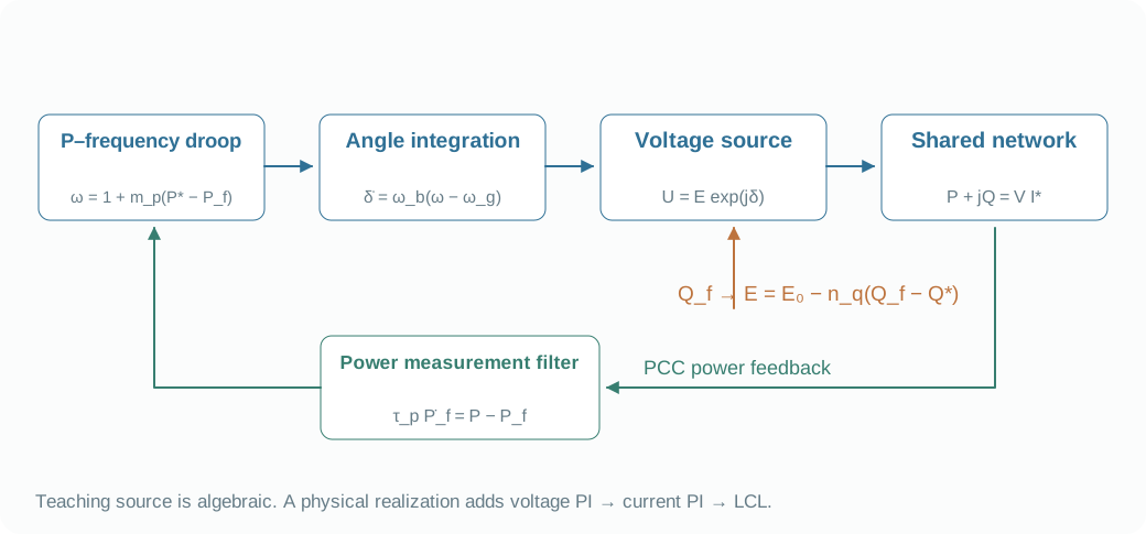
\tau_p\dot P_f=P_{PoC}-P_f,\qquad\tau_q\dot Q_f=Q_{PoC}-Q_f\omega=1-m_p(P_f-P^*),\quad E=E_0-n_q(Q_f-Q^*),\quad\dot\delta=\omega_b(\omega-\omega_g)I=\frac{Ee^{j\delta}-V}{Z_f},\qquad P+jQ=VI^*05.02 MECHANISM & DERIVATION
Distinguish the terminal target from the raw command
At a nominal-frequency locked equilibrium, P_f = P*. Reactive matching is subtler. The internal source amplitude must support the voltage drop across Z_f. With E₀ fixed at 1, Q* must compensate that required amplitude even when terminal Q is zero.
At SCR = 5, the default matched Q* is approximately 0.316795 pu while PoC Q = 0. This is a controller offset. Forcing every controller to use the same raw Q* would silently change the operating point and compromise the comparison.
05.03 MECHANISM & DERIVATION
A frequency event reveals the steady slope
At a new locked equilibrium, internal frequency equals grid frequency. Rearranging the droop law predicts P = P* − (ω_g − 1)/m_p. A +0.1 Hz event at 50 Hz is +0.002 pu, so m_p = 0.02 predicts a −0.1 pu power change.
The same m_p also affects transient loop gain. With fixed τ_p = 0.1 s and τ_q = 0.05 s, changes in peak or damping reflect network, filter and control interactions. A steady slope alone does not determine the transient.
05.04 MECHANISM & DERIVATION
Restore the cascaded loops when the question requires them
A detailed implementation sets v* = [E,0]. Voltage PI, output-current feedforward and capacitor decoupling create i₁*. Current PI then creates u for the LCL plant. F is the output-current feedforward gain; K_p and K_i denote the corresponding PI gains. Six electrical states, four integrators, two power filters and one angle give 13 states.
The canonical source filters power measured using v_c and i₂, whereas benchmark outputs are reconstructed at PoC. The browser lab deliberately uses PoC feedback. When reproducing the detailed source, preserve its measurement port and initialize PI integrals to support the equilibrium voltage and current; zero tracking error does not imply zero integrator state.
At a no-limit equilibrium with zero voltage and current errors, solve the two PI equations for their integrals. The nonzero offsets below support the required capacitor current and converter voltage. Setting the integrators to zero would turn an equilibrium comparison into an unintended startup transient.
e_v=v^*-v_c,\quad\dot\xi_v=e_v,\quad i_1^*=F i_2-\omega_b\omega cJv_c+K_{pv}e_v+K_{iv}\xi_ve_i=i_1^*-i_1,\quad\dot\xi_i=e_i,\quad u=v_c-\omega_b\omega\ell_1Ji_1+K_{pi}e_i+K_{ii}\xi_i\xi_v=\frac{i_1-Fi_2+\omega_b\omega cJv_c}{K_{iv}},\qquad\xi_i=\frac{u-v_c+\omega_b\omega\ell_1Ji_1}{K_{ii}}FROM EQUATION TO JUDGMENT
Work the case
Let P* = 0.6 pu and m_p = 0.02. The grid rises from 50 to 50.1 Hz. Predict the locked steady power.
- The per-unit frequency increase is 0.1/50 = 0.002.
- The droop power reduction is 0.002/0.02 = 0.1 pu.
- Subtract that reduction from the reference 0.6 pu.
The predicted locked power is 0.5 pu. The calculation assumes the stated model reaches the new equilibrium.
FROM PREDICTION TO EVIDENCE
Power changes through angle motion
The +0.03 pu P* step first creates a frequency mismatch, then increases transferred power. The transient reveals filter and network feedback.
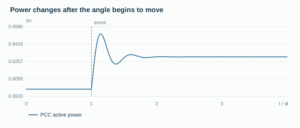
- At the command step, the filtered power cannot jump, so frequency changes first.
- Advancing source angle increases power through the network; measured power feeds back.
- The nominal-frequency equilibrium requires P = P*; inspect the window before calling it settled.
Your experiment
- Run +0.03 pu P*, then inspect frequency: explain why it changes before power settles.
- Inspect the matched Q* and compare it with measured Q at time zero.
- Apply +0.1 Hz and compare the final P change with −0.1/(50 m_p).
Laboratory · Python runs in your browser
Predict → run → inspect
Predict the response, then change a parameter and run. The initial plot is a baseline generated by the same solver. The first computation downloads Python; later runs reuse it.
Loading the baseline…
Numerical audit and samples
Low-frequency teaching realization: nominal-frequency algebraic network and ideal current/voltage realization. 50 Hz, 10 kVA, 400 V; initial PCC total P = 0.6, Q = 0; X/R = 10. τᵢ = 0.02 s, τₚ = 0.1 s, τq = 0.05 s, nq = 0.0325; GFM source impedance 0.00625 + j0.1 pu. LCL, inner PI, DC dynamics and current limits are omitted.
CHECK YOUR REASONING
Can you explain it—and calculate it?
Your engineering decision
Use one command step and one frequency step to separate transient mechanism from steady slope. Explain why this droop source needs no PLL in its synchronization law.
REPRODUCE & EXTEND
Take the evidence into your model
Core equation reference
\tau_p\dot P_f=P_{PoC}-P_f,\qquad\tau_q\dot Q_f=Q_{PoC}-Q_f\omega=1-m_p(P_f-P^*),\quad E=E_0-n_q(Q_f-Q^*),\quad\dot\delta=\omega_b(\omega-\omega_g)I=\frac{Ee^{j\delta}-V}{Z_f},\qquad P+jQ=VI^*e_v=v^*-v_c,\quad\dot\xi_v=e_v,\quad i_1^*=F i_2-\omega_b\omega cJv_c+K_{pv}e_v+K_{iv}\xi_ve_i=i_1^*-i_1,\quad\dot\xi_i=e_i,\quad u=v_c-\omega_b\omega\ell_1Ji_1+K_{pi}e_i+K_{ii}\xi_i\xi_v=\frac{i_1-Fi_2+\omega_b\omega cJv_c}{K_{iv}},\qquad\xi_i=\frac{u-v_c+\omega_b\omega\ell_1Ji_1}{K_{ii}}Open the Python experiment and model source
The code reads the lab parameters and draws its own result. Edit the experiment or source to test your prediction. Download a single .py file with parameters, solver and experiment; local execution requires Python 3.
case is a snapshot of the controls when you press Run. Call solve(case) and assign the final solution to result to plot it.
The first run needs internet access to download Python. Computation stays in your browser; the solver uses only the standard library.
Ready to run.
Output appears here.
Python result
Inspect and edit the model source (advanced)
Source edits affect the next Python experiment; the lab above retains the original teaching equations.
Source materials and model scope
Based on local PINN-IBR materials reviewed on 2026-10-03. The website uses independent teaching realizations; low-frequency models retain nominal-frequency algebraic networks and ideal actuators. Continue into the detailed models below.
Coding/Modeling/src/ibrsim/models/droop_gfm.pyCoding/Modeling/Single-IBR-Infinite-Bus/00_Droop_GFM_Infinite_Bus_Model_Library.ipynb
WHAT FOLLOWS
Droop sets frequency algebraically. The next lesson adds a speed state and asks what virtual inertia changes—and what evidence it leaves unresolved.