LESSON 04 / 09 · MODELING & SIMULATION
PLL and Grid-Following Control
When the grid angle moves, what does GFL follow?
THE CASE
When the grid angle moves, what does GFL follow?
The grid frequency rises by 0.1 Hz. The current controller still receives the same power request. Trace the causal chain from measured voltage, through PLL angle, to current injection before predicting the response.
By the end of this lesson, you should be able to…
- Explain how a PLL establishes the local reference frame.
- Derive the power-to-current and current-control paths.
04.01 MECHANISM & DERIVATION
Acquire an angle before requesting current
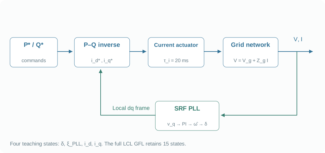
The SRF PLL expresses terminal voltage in its estimated frame and drives local v_q toward zero. Positive v_q means the voltage vector leads the estimated d axis; increasing the estimated angle closes that error. The power request is then converted into local current and rotated into the network frame.
The four-state teaching model retains relative PLL angle δ, integral ξ and two current-actuator components. A 20 ms ideal actuator replaces the current PI and LCL plant. This isolates synchronization and power tracking while removing the fast electrical dynamics from Lesson 3.
04.02 MECHANISM & DERIVATION
Translate a design frequency into PLL gains
Normalize the detector as e = v_q/|V| and define the PI output as per-unit frequency. Multiplication by ω_b occurs in the relative-angle equation. Near alignment with a stiff voltage, the characteristic polynomial is s² + ω_bk_p s + ω_bk_i.
Matching it to s² + 2ζω_n s + ω_n² gives the gains below. The lab uses ζ = 0.707 and ω_n = 2πb. Thus b is a natural-frequency design parameter in Hz; network feedback means it need not equal the measured closed-loop −3 dB bandwidth.
e=\frac{v_q}{\lVert v\rVert},\quad\dot\xi=e,\quad\hat\omega=1+k_pe+k_i\xi,\quad\dot\delta=\omega_b(\hat\omega-\omega_g)k_p=\frac{2\zeta\omega_n}{\omega_b},\qquad k_i=\frac{\omega_n^2}{\omega_b}04.03 MECHANISM & DERIVATION
Close the feedback through the grid impedance
The exact inverse P–Q map uses both measured voltage components. The network then returns V = V_g + Z_gI. Because the same voltage feeds the PLL, current injection affects the controller’s own angle measurement. Reducing SCR strengthens this interaction.
For the stated +0.1 Hz event, the PLL should track the new frequency. This teaching controller contains no frequency–watt or RoCoF power law, so frequency tracking alone does not imply a changed steady P request. Compare estimated frequency, P and PCC voltage together before drawing a conclusion.
\tau_i\dot i_{dq}=i_{dq}^*-i_{dq},\qquad V=V_g+Z_gI04.04 MECHANISM & DERIVATION
Reconnect the physical current controller
The detailed LCL realization first maps PoC power to i₂*. Capacitor-current compensation creates i₁*, and current PI with voltage feedforward and inductive decoupling generates converter voltage u. The plant equations then determine the actual current.
The full 15-state GFL has one angle, one PLL integral, two voltage measurements, one frequency measurement, two power-command filters, two current PI integrators and six electrical states. A bounded four-state response therefore cannot establish the detailed model’s inner-loop stability.
i_1^*=i_2^*-\omega_b\hat\omega cJv_c,\quad\dot\xi_i=i_1^*-i_1u=v_c-\omega_b\hat\omega\ell_1Ji_1+K_{pi}(i_1^*-i_1)+K_{ii}\xi_iFROM EQUATION TO JUDGMENT
Work the case
Use b = 2 Hz, ζ = 0.707 and f_b = 50 Hz. Calculate the proportional gain for the normalized PLL.
- The natural angular frequency is ω_n = 2π × 2.
- The base angular frequency is ω_b = 2π × 50.
- Substitute into k_p = 2ζω_n/ω_b; the factors 2π cancel.
k_p = 0.05656. Changing the detector normalization or PI output units would require changing this gain.
FROM PREDICTION TO EVIDENCE
Frequency tracking is an angle-estimation task
For this figure, grid frequency rises 0.1 Hz at 1 s. The PLL estimate converges; the live lab below starts with a P-command baseline.
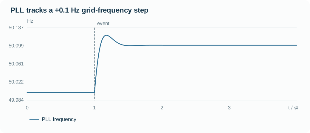
- At 1 s, the grid frequency rises; angle error drives the PLL correction.
- The temporary frequency overshoot belongs to the angle-estimation feedback.
- The estimate converges to 50.1 Hz; unchanged P* supplies no frequency–watt response in this model.
Your experiment
- Run the baseline P step, then select estimated frequency and PCC magnitude.
- Apply a +0.1 Hz grid-frequency step; check the PLL frequency after the transient.
- At SCR = 2, compare PLL design settings of 1 and 5 Hz using the same disturbance.
Laboratory · Python runs in your browser
Predict → run → inspect
Predict the response, then change a parameter and run. The initial plot is a baseline generated by the same solver. The first computation downloads Python; later runs reuse it.
Loading the baseline…
Numerical audit and samples
Low-frequency teaching realization: nominal-frequency algebraic network and ideal current/voltage realization. 50 Hz, 10 kVA, 400 V; initial PCC total P = 0.6, Q = 0; X/R = 10. τᵢ = 0.02 s, τₚ = 0.1 s, τq = 0.05 s, nq = 0.0325; GFM source impedance 0.00625 + j0.1 pu. LCL, inner PI, DC dynamics and current limits are omitted.
CHECK YOUR REASONING
Can you explain it—and calculate it?
Your engineering decision
At SCR = 5, predict a +0.1 Hz event before running it. Then reduce SCR to 2 and explain changes through voltage–current–PLL feedback, rather than through the GFL label alone.
REPRODUCE & EXTEND
Take the evidence into your model
Core equation reference
e=\frac{v_q}{\lVert v\rVert},\quad\dot\xi=e,\quad\hat\omega=1+k_pe+k_i\xi,\quad\dot\delta=\omega_b(\hat\omega-\omega_g)k_p=\frac{2\zeta\omega_n}{\omega_b},\qquad k_i=\frac{\omega_n^2}{\omega_b}\tau_i\dot i_{dq}=i_{dq}^*-i_{dq},\qquad V=V_g+Z_gIi_1^*=i_2^*-\omega_b\hat\omega cJv_c,\quad\dot\xi_i=i_1^*-i_1u=v_c-\omega_b\hat\omega\ell_1Ji_1+K_{pi}(i_1^*-i_1)+K_{ii}\xi_iOpen the Python experiment and model source
The code reads the lab parameters and draws its own result. Edit the experiment or source to test your prediction. Download a single .py file with parameters, solver and experiment; local execution requires Python 3.
case is a snapshot of the controls when you press Run. Call solve(case) and assign the final solution to result to plot it.
The first run needs internet access to download Python. Computation stays in your browser; the solver uses only the standard library.
Ready to run.
Output appears here.
Python result
Inspect and edit the model source (advanced)
Source edits affect the next Python experiment; the lab above retains the original teaching equations.
Source materials and model scope
Based on local PINN-IBR materials reviewed on 2026-10-03. The website uses independent teaching realizations; low-frequency models retain nominal-frequency algebraic networks and ideal actuators. Continue into the detailed models below.
Coding/Modeling/src/ibrsim/models/gfl_pll_pq_droop.pyCoding/Modeling/Single-IBR-Infinite-Bus/02_GFL_PLL_PQDroop_Infinite_Bus.ipynb
WHAT FOLLOWS
GFL acquires its angle from voltage. The next controller creates its own angle from a power mismatch and closes synchronization through the network.