LESSON 01 / 09 · MODELING & SIMULATION
System Boundaries and Model Representations
Which model is sufficient for the decision?
THE CASE
Which model is sufficient for the decision?
A project team has four plausible inverter models and four different step responses. Before choosing a controller, the team must decide what each response can legitimately explain. Begin with the decision, then define the model boundary.
By the end of this lesson, you should be able to…
- Distinguish states, inputs, outputs, and algebraic variables.
- Declare the model boundary and study objective.
01.01 MECHANISM & DERIVATION
Start with the consequence you need to explain
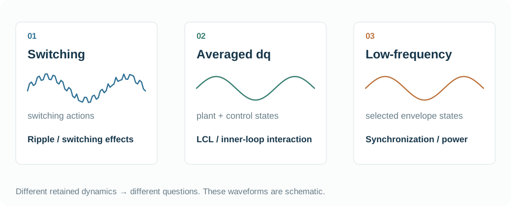
A converter can be studied over switching cycles, electrical transients or slower synchronization dynamics. These are different questions about the same equipment. If the concern is switching ripple, the switching events matter. If it is an LCL oscillation, stored electrical energy matters. If it is a small power-command response over seconds, a reduced synchronization model may be enough.
The modeling decision is therefore a tradeoff between retained mechanisms and the evidence needed for a decision. State the output, disturbance and time horizon before selecting a controller family. “GFM” identifies a control concept; it does not specify model order.
01.02 MECHANISM & DERIVATION
Draw the terminal before counting states
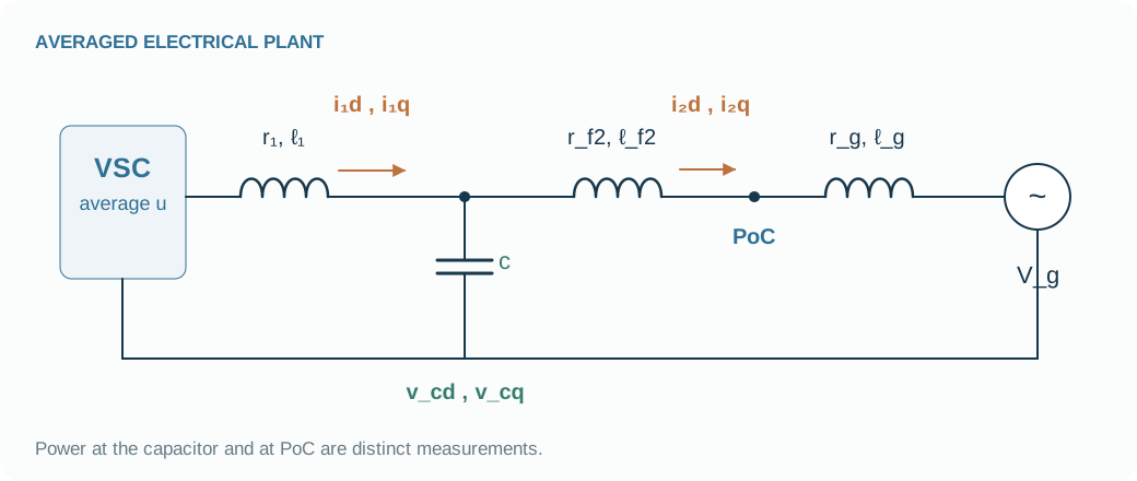
Trace the physical chain from average converter voltage through L₁, the capacitor, L₂ and the point of connection to the grid impedance and infinite bus. The capacitor port and PoC are separated by a branch that stores energy and dissipates power. A power value without a measurement port is incomplete.
In this course, injected current points toward the grid; positive P and Q denote injection at the declared port. The infinite bus sets voltage and frequency and the DC source is ideal. These assumptions define what the experiment can tell us about an interconnection.
01.03 MECHANISM & DERIVATION
Turn the boundary into a model contract
Partition the model into differential states x, algebraic network variables z, inputs u and outputs y. A quantity is a state because it has an evolution law, not because it appears on a plot. The network constraint must agree with the controller at every time sample.
For the three-state droop experiment, x = [δ, P_f, Q_f]. PCC voltage and branch current are algebraic; power references and grid conditions are inputs. Capacitor voltage is absent. This immediately explains why that model cannot reproduce the six-state LCL resonance studied in Lesson 3.
\dot{x}=f(x,z,u),\qquad 0=g(x,z,u),\qquad y=h(x,z,u)FROM EQUATION TO JUDGMENT
Work the case
A detailed droop realization retains 13 states. The browser droop realization retains 3. What did the reduction remove?
- Count the six electrical states: two components each for i₁, v_c and i₂.
- Count four PI integrators: two voltage-loop and two current-loop integrators.
- The remaining angle and two power filters are the three reduced states.
13 − 3 = 10 states were removed. The reduction removes electrical storage and inner-control dynamics; it does not merely shorten a vector.
FROM PREDICTION TO EVIDENCE
Same terminal, different trajectories
All four families start at P = 0.6 pu and Q = 0. A +0.03 pu command at 1 s exposes their retained dynamics.
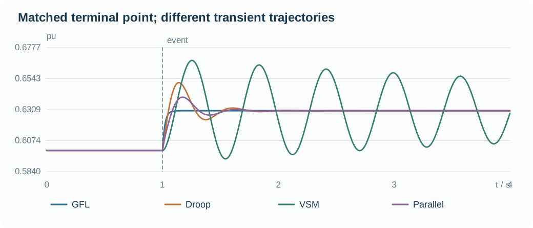
- Before the event, all four traces agree at 0.6 pu: the terminal target has been matched.
- After the event, their paths diverge because their retained synchronization and actuator dynamics differ.
- The absence of LCL states means none of these four curves can explain the plant resonance.
Your experiment
- Run the default comparison and identify which dynamics are retained in each trace.
- Choose a voltage step and explain why these traces cannot establish switching-ripple accuracy.
- Write a four-line model contract: boundary, states, inputs, measured outputs.
Laboratory · Python runs in your browser
Predict → run → inspect
Predict the response, then change a parameter and run. The initial plot is a baseline generated by the same solver. The first computation downloads Python; later runs reuse it.
Loading the baseline…
Numerical audit and samples
Low-frequency teaching realization: nominal-frequency algebraic network and ideal current/voltage realization. 50 Hz, 10 kVA, 400 V; initial PCC total P = 0.6, Q = 0; X/R = 10. τᵢ = 0.02 s, τₚ = 0.1 s, τq = 0.05 s, nq = 0.0325; GFM source impedance 0.00625 + j0.1 pu. LCL, inner PI, DC dynamics and current limits are omitted.
CHECK YOUR REASONING
Can you explain it—and calculate it?
Your engineering decision
Write a four-line model contract: question, port, retained states and excluded mechanisms. Use it to qualify any conclusion drawn from the four-family plot.
REPRODUCE & EXTEND
Take the evidence into your model
Core equation reference
\dot{x}=f(x,z,u),\qquad 0=g(x,z,u),\qquad y=h(x,z,u)Open the Python experiment and model source
The code reads the lab parameters and draws its own result. Edit the experiment or source to test your prediction. Download a single .py file with parameters, solver and experiment; local execution requires Python 3.
case is a snapshot of the controls when you press Run. Call solve(case) and assign the final solution to result to plot it.
The first run needs internet access to download Python. Computation stays in your browser; the solver uses only the standard library.
Ready to run.
Output appears here.
Python result
Inspect and edit the model source (advanced)
Source edits affect the next Python experiment; the lab above retains the original teaching equations.
Source materials and model scope
Based on local PINN-IBR materials reviewed on 2026-10-03. The website uses independent teaching realizations; low-frequency models retain nominal-frequency algebraic networks and ideal actuators. Continue into the detailed models below.
Teaching/Tutorial-IBR/src/tutorial_en.texCoding/Modeling/Single-IBR-Infinite-Bus/README.md
WHAT FOLLOWS
With the boundary fixed, the next risk is convention: two correct-looking equations can describe different quantities if coordinates and bases differ.