LESSON 06 / 09 · MODELING & SIMULATION
VSM and Virtual Inertia
What does virtual inertia actually change?
THE CASE
What does virtual inertia actually change?
A design review proposes doubling virtual inertia to improve the response. Before accepting the claim, distinguish initial rate, oscillatory behavior, steady power and physical energy capability.
By the end of this lesson, you should be able to…
- Read a VSM swing equation and its static droop relation.
- Separate requested support from delivered power.
06.01 MECHANISM & DERIVATION
Add a speed state with an explicit evolution law
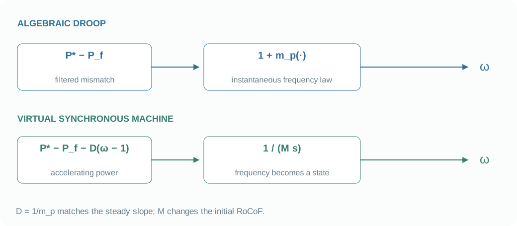
The VSM replaces algebraic frequency droop with Mω̇ = P* − P_f − D(ω − 1). It retains δ, ω, P_f and Q_f. The electrical source and reactive law are the same as in the droop lab, so the comparison isolates the synchronization law.
Use M in seconds and D = 1/m_p. Under this swing convention M = 2H; the default M = 4 s corresponds to H = 2 s. The source repository separates governor and explicit damping contributions, while the teaching model uses their aggregate coefficient.
M\dot\omega=P^*-P_f-D(\omega-1),\qquad D=\frac1{m_p},\qquad M=2H06.02 MECHANISM & DERIVATION
Separate initial rate from steady sharing
Immediately after a P* step, speed and filtered power still equal their old equilibrium values. The accelerating mismatch is therefore ΔP*, so ḟ = f_bΔP*/M. Doubling M halves this initial rate under the same conditions.
At equilibrium ω̇ = 0 and ω = ω_g. The power–frequency slope then equals droop when D = 1/m_p, independent of M. Larger inertia can change oscillation and settling through its interaction with the 0.1 s power filter; it is not a general guarantee of a better trajectory.
\dot\delta=\omega_b(\omega-\omega_g),\qquad P_{\infty}=P^*-\frac{\omega_g-1}{m_p}\dot f(1^+)=f_b\frac{\Delta P^*}{M}06.03 MECHANISM & DERIVATION
Translate the control law into evidence requirements
Virtual inertia describes a controller. Delivering its requested power requires a DC energy source, available current and a feasible converter voltage. The lab assumes an ideal DC supply and unlimited realization; it cannot establish those hardware capabilities.
A PLL-based GFL can also add filtered RoCoF power support while remaining grid-following. That structure differs from a VSM internal speed state. The source GFL-VI notebook includes an unstable frozen-parameter case, illustrating why an inertia-labelled term alone does not establish stability.
FROM EQUATION TO JUDGMENT
Work the case
A +0.03 pu power-reference step occurs at equilibrium. Use M = 4 s and a 50 Hz base to calculate initial RoCoF.
- The speed derivative is 0.03/4 = 0.0075 pu/s.
- Multiply by 50 Hz to convert to physical frequency rate.
- Repeating with M = 8 s gives half the initial rate.
Initial RoCoF is 0.375 Hz/s. This local prediction says nothing by itself about settling time or energy availability.
FROM PREDICTION TO EVIDENCE
The same slope does not imply the same transient
Droop and VSM share source, filters and slope. Only the frequency law differs here; the 4 s window need not capture settling.
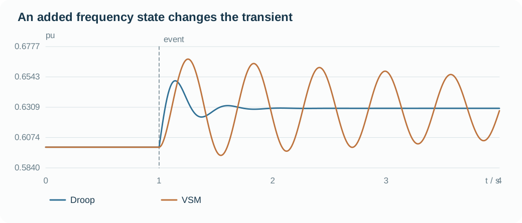
- Both cases receive the same power command and share source, filters and steady slope.
- VSM speed cannot jump: the added state changes the early trajectory and oscillatory response.
- The end of a 4 s plot is a last sample, not automatically a settled value.
Your experiment
- With M = 4 s, predict the initial frequency derivative for a +0.03 pu step.
- Repeat at M = 1 and 8 s while holding m_p and SCR fixed.
- Use the frequency-step experiment to compare the steady slope with droop GFM.
Laboratory · Python runs in your browser
Predict → run → inspect
Predict the response, then change a parameter and run. The initial plot is a baseline generated by the same solver. The first computation downloads Python; later runs reuse it.
Loading the baseline…
Numerical audit and samples
Low-frequency teaching realization: nominal-frequency algebraic network and ideal current/voltage realization. 50 Hz, 10 kVA, 400 V; initial PCC total P = 0.6, Q = 0; X/R = 10. τᵢ = 0.02 s, τₚ = 0.1 s, τq = 0.05 s, nq = 0.0325; GFM source impedance 0.00625 + j0.1 pu. LCL, inner PI, DC dynamics and current limits are omitted.
CHECK YOUR REASONING
Can you explain it—and calculate it?
Your engineering decision
Compare M = 1, 4 and 8 s with the same slope and filters. Report initial rate, peak and whether settling is visible. Extend the window to 20 s before claiming a steady value; keep growing oscillations in the report.
REPRODUCE & EXTEND
Take the evidence into your model
Core equation reference
M\dot\omega=P^*-P_f-D(\omega-1),\qquad D=\frac1{m_p},\qquad M=2H\dot\delta=\omega_b(\omega-\omega_g),\qquad P_{\infty}=P^*-\frac{\omega_g-1}{m_p}\dot f(1^+)=f_b\frac{\Delta P^*}{M}Open the Python experiment and model source
The code reads the lab parameters and draws its own result. Edit the experiment or source to test your prediction. Download a single .py file with parameters, solver and experiment; local execution requires Python 3.
case is a snapshot of the controls when you press Run. Call solve(case) and assign the final solution to result to plot it.
The first run needs internet access to download Python. Computation stays in your browser; the solver uses only the standard library.
Ready to run.
Output appears here.
Python result
Inspect and edit the model source (advanced)
Source edits affect the next Python experiment; the lab above retains the original teaching equations.
Source materials and model scope
Based on local PINN-IBR materials reviewed on 2026-10-03. The website uses independent teaching realizations; low-frequency models retain nominal-frequency algebraic networks and ideal actuators. Continue into the detailed models below.
Coding/Modeling/src/ibrsim/models/vsm_gfm.pyCoding/Modeling/Single-IBR-Infinite-Bus/06_VSM_GFM_Infinite_Bus.ipynbCoding/Modeling/Single-IBR-Infinite-Bus/04_GFL_PLL_Virtual_Inertia_Infinite_Bus.ipynb
WHAT FOLLOWS
We have two distinct synchronization mechanisms. The next lesson couples them simultaneously at one PCC, where their interactions become part of the model.