LESSON 09 / 09 · MODELING & SIMULATION
Equilibrium, Disturbances, and Fair Comparison
What evidence makes a model comparison credible?
THE CASE
What evidence makes a model comparison credible?
A review panel asks which controller is best. Four attractive curves are insufficient: the starting point, event, observation port and numerical accuracy must agree before the differences mean anything.
By the end of this lesson, you should be able to…
- Solve a matched point-of-connection operating point.
- Preserve failed or unstable cases in the comparison.
09.01 MECHANISM & DERIVATION
Match the physical target, not every input number
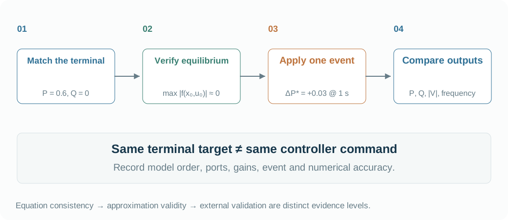
Use one 10 kVA, 400 V, 50 Hz base, one PoC and one grid. Set total initial P = 0.6 pu and Q = 0; the parallel case splits that target between branches. Solve S = VI* with V = 1 + Z_gI, selecting the high-voltage power-flow root.
Each controller must realize this point in its own coordinates. Droop and VSM need Q* offsets to support their internal voltage drop. Different raw commands can therefore produce the same physical target, which is the comparison we need.
S=VI^*,\qquad V=1+Z_g\overline{S/V},\qquad\lVert f(x_0,u_0)\rVert_\infty<\varepsilonZ_g=\frac{1+j\,10}{\mathrm{SCR}\sqrt{101}},\qquad\Delta P^*_{branch}=\frac{\Delta P^*_{total}}{N}09.02 MECHANISM & DERIVATION
Verify equilibrium and place events exactly
Check max|f(x₀,u₀)| before applying a disturbance. Integrate up to 1 s under the old input, then start a new segment under the changed input. Duplicate-time samples capture before and after values without averaging a discontinuity across Runge–Kutta stages.
The default step is 0.5 ms. Repeat with 0.25 ms and compare trajectories on the same output grid. A smooth line is a rendering property; refinement is evidence about the numerical solution. Switching cases need an additional segment boundary and reset at 2 s.
e_h=\max_k|P_h(t_k)-P_{h/2}(t_k)|09.03 MECHANISM & DERIVATION
Separate consistency, validity and validation
Equilibrium, KCL, power sums and reset residuals establish consistency with the stated equations. Comparing against a higher-order realization over a declared range assesses approximation validity. Independent measurements or a qualified reference are needed for external validation.
The browser experiments provide the first kind of evidence. Retain unstable results rather than hiding them. Extend the 4 s window when VSM settling is unresolved. Conclusions should identify the model, disturbance and parameter range instead of announcing a global controller ranking.
09.04 MECHANISM & DERIVATION
Turn the comparison into a decision brief
Submit a short brief with a model contract, matched-equilibrium table, two controlled disturbances and an explanation of the observed differences. Attach the parameter snapshot, executable experiment and a refinement check.
End with a recommendation proportional to the evidence: which realization is sufficient for the stated study, what mechanism explains its response, and which additional dynamics must be tested before extending the conclusion. The full-order source notebooks offer the next level of investigation.
FROM EQUATION TO JUDGMENT
Work the case
For an equilibrium illustration, required source E is 1.01 pu, E₀ = 1, terminal Q = 0 and n_q = 0.0325. Find the matching Q*.
- At equilibrium, Q_f = terminal Q = 0.
- Rearrange E = E₀ − n_q(Q_f − Q*).
- Thus Q* = (1.01 − 1)/0.0325.
The matching command is 0.307692 pu despite zero terminal Q. The given source amplitude is illustrative, not the default SCR = 5 amplitude.
FROM PREDICTION TO EVIDENCE
Curves become evidence only after the protocol
Matched PoC power and an identical total command step isolate the stated model differences. The overlay does not establish a universal ranking.
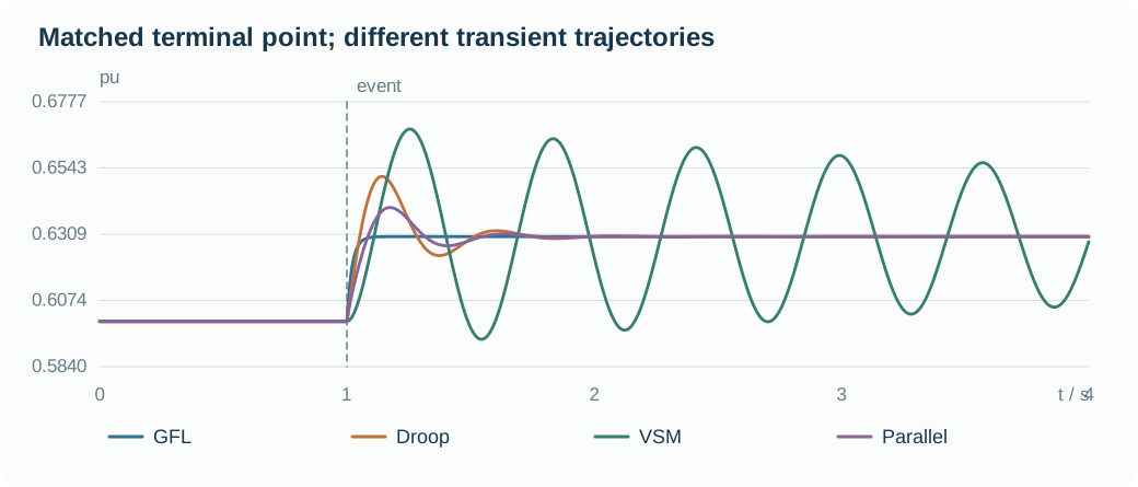
- All cases begin at the same total PoC P and Q, even though raw commands differ.
- One total command step exposes the model-specific transient mechanisms.
- Inspect equilibrium and timestep refinement before attributing a difference to control design.
Your experiment
- Compare all four models at SCR = 5 with the +0.03 pu total P step.
- Repeat with a +0.1 Hz frequency step; explain the GFL versus GFM steady responses.
- In Python, halve case["dt"] and compare aligned samples; retain the maximum error in the report.
Laboratory · Python runs in your browser
Predict → run → inspect
Predict the response, then change a parameter and run. The initial plot is a baseline generated by the same solver. The first computation downloads Python; later runs reuse it.
Loading the baseline…
Numerical audit and samples
Low-frequency teaching realization: nominal-frequency algebraic network and ideal current/voltage realization. 50 Hz, 10 kVA, 400 V; initial PCC total P = 0.6, Q = 0; X/R = 10. τᵢ = 0.02 s, τₚ = 0.1 s, τq = 0.05 s, nq = 0.0325; GFM source impedance 0.00625 + j0.1 pu. LCL, inner PI, DC dynamics and current limits are omitted.
CHECK YOUR REASONING
Can you explain it—and calculate it?
Your engineering decision
Prepare a two-page decision brief. Give equal attention to the model contract, derivation, experiment and strength of evidence; include unresolved limits in the recommendation.
REPRODUCE & EXTEND
Take the evidence into your model
Core equation reference
S=VI^*,\qquad V=1+Z_g\overline{S/V},\qquad\lVert f(x_0,u_0)\rVert_\infty<\varepsilonZ_g=\frac{1+j\,10}{\mathrm{SCR}\sqrt{101}},\qquad\Delta P^*_{branch}=\frac{\Delta P^*_{total}}{N}e_h=\max_k|P_h(t_k)-P_{h/2}(t_k)|Open the Python experiment and model source
The code reads the lab parameters and draws its own result. Edit the experiment or source to test your prediction. Download a single .py file with parameters, solver and experiment; local execution requires Python 3.
case is a snapshot of the controls when you press Run. Call solve(case) and assign the final solution to result to plot it.
The first run needs internet access to download Python. Computation stays in your browser; the solver uses only the standard library.
Ready to run.
Output appears here.
Python result
Inspect and edit the model source (advanced)
Source edits affect the next Python experiment; the lab above retains the original teaching equations.
Source materials and model scope
Based on local PINN-IBR materials reviewed on 2026-10-03. The website uses independent teaching realizations; low-frequency models retain nominal-frequency algebraic networks and ideal actuators. Continue into the detailed models below.
Coding/Modeling/Single-IBR-Infinite-Bus/12_Single_IBR_Control_Family_Comparison.ipynbResearch-Xirui-Zhang/Coding/xirui_low_frequency/model.py
WHAT FOLLOWS
The modeling course ends here. A physics-informed or neural-ODE surrogate should inherit this same state definition, port convention, equilibrium and event protocol.