LESSON 02 / 09 · MODELING & SIMULATION
Reference Frames and Per-Unit Conventions
How can rotating coordinates preserve the same physics?
THE CASE
How can rotating coordinates preserve the same physics?
Two engineers report different dq currents for the same three-phase waveform. One reports positive reactive injection with positive i_q; the other uses negative i_q. Resolve the convention before blaming either controller.
By the end of this lesson, you should be able to…
- Apply a declared dq transform and power convention.
- Check angle, frequency, and time units.
02.01 MECHANISM & DERIVATION
Rotate the description, preserve the power
A balanced waveform becomes almost constant in a frame rotating with it. This makes electrical and control dynamics easier to interpret. The course uses a power-invariant Park transform with √(2/3) scaling, cosine d row and negative-sine q row.
On the balanced subspace, the transpose gives the inverse. Because this transform preserves the inner product, P has no additional 3/2 factor. A zero-sequence component requires another axis. Mixing transform conventions creates an error even if each borrowed equation was correct in its original setting.
T(\theta)=\sqrt{\frac{2}{3}}\begin{bmatrix}\cos\theta&\cos(\theta-2\pi/3)&\cos(\theta+2\pi/3)\\-\sin\theta&-\sin(\theta-2\pi/3)&-\sin(\theta+2\pi/3)\end{bmatrix}02.02 MECHANISM & DERIVATION
Derive the current request from the measured voltage
With injection-positive current, P = v_d i_d + v_q i_q and Q = v_q i_d − v_d i_q. If the d axis aligns with voltage, positive Q requires negative i_q. This sign is a direct consequence of the chosen q axis.
Invert both equations together to obtain the current reference. The full inverse remains valid while the PLL is misaligned, provided voltage magnitude is nonzero. Replacing it with i_d = P/v_d and i_q = −Q/v_d assumes v_q = 0 throughout the transient—a stronger assumption than the controller actually guarantees.
P=v_d i_d+v_q i_q,\qquad Q=v_q i_d-v_d i_q\begin{bmatrix}i_d^*\\i_q^*\end{bmatrix}=\frac{1}{v_d^2+v_q^2}\begin{bmatrix}v_d&v_q\\v_q&-v_d\end{bmatrix}\begin{bmatrix}P^*\\Q^*\end{bmatrix}02.03 MECHANISM & DERIVATION
Keep the dimensions underneath per unit
Use 10 kVA, 400 V line-to-line RMS and 50 Hz. Then Z_b = 16 Ω, the power-invariant dq voltage base is 400 V, and the dq current base is 25 A. The line RMS current base is 14.434 A; these two current quantities must not be substituted for one another.
The dynamic coefficients ℓ = L/Z_b and c = CZ_b have units of seconds. Nominal reactance x = ω_bℓ is a different quantity. Likewise, a per-unit frequency difference needs multiplication by ω_b before it becomes an angle rate. Units are a practical way to catch plausible-looking modeling errors.
Z_b=\frac{V_b^2}{S_b},\quad I_{b,dq}=\frac{S_b}{V_b},\quad \dot\delta=\omega_b(\omega_{pu}-\omega_{g,pu})FROM EQUATION TO JUDGMENT
Work the case
The base frequency is 50 Hz and the relative frequency difference is 0.001 pu. Determine the angle drift rate.
- Convert the frequency difference: 50 × 0.001 = 0.05 Hz.
- Convert cycles to radians: 2π × 0.05.
- Use this rate in the relative-angle differential equation.
The angle rate is 0.314159 rad/s. Over one second the relative angle advances about 18°, which is large enough to matter to a synchronizing controller.
FROM PREDICTION TO EVIDENCE
Components change; power does not
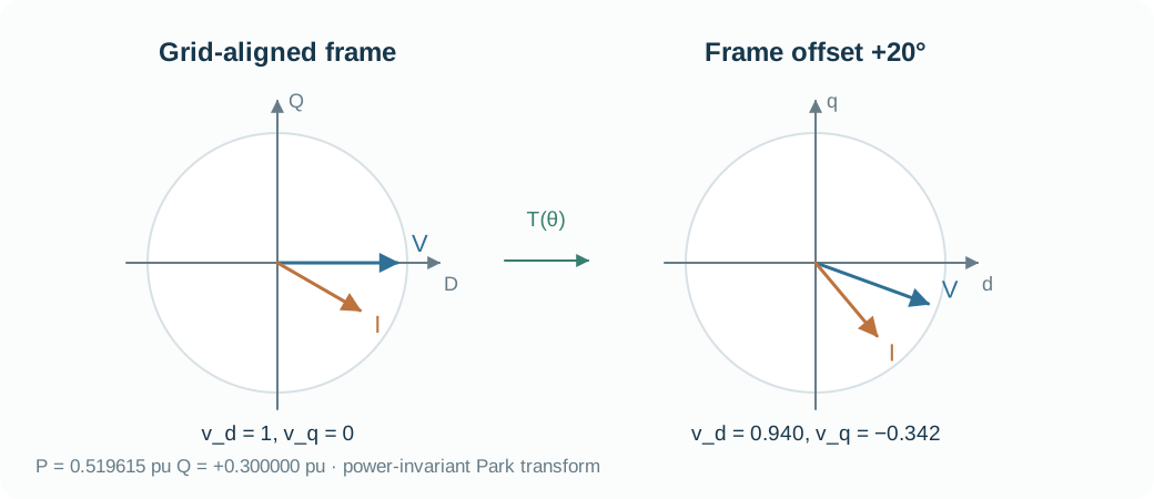
The fixed 20° offset rotates both vectors. Read constant P and Q as the invariant, not constant voltage components across frames.
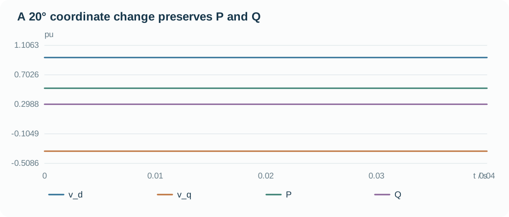
- At +20°, voltage has a nonzero q component even though the physical voltage is unchanged.
- Voltage and current rotate together, so their power inner product remains invariant.
- Change the angle in the lab and check both P and Q, rather than only one coordinate component.
Your experiment
- Set the frame offset to 0°, +20° and −90°; compare v_d and v_q.
- Select the P–Q plot and verify that the physical power is invariant.
- Edit the current lag in frame_run() and predict the signs of P and Q before running.
Laboratory · Python runs in your browser
Predict → run → inspect
Predict the response, then change a parameter and run. The initial plot is a baseline generated by the same solver. The first computation downloads Python; later runs reuse it.
Loading the baseline…
Numerical audit and samples
Balanced, power-invariant transform without zero sequence. P and Q use the common base.
CHECK YOUR REASONING
Can you explain it—and calculate it?
Your engineering decision
Rotate both voltage and current by 20°. Explain why v_d and v_q change while P and Q remain fixed. Record the Park normalization and current direction beside every dq plot.
REPRODUCE & EXTEND
Take the evidence into your model
Core equation reference
T(\theta)=\sqrt{\frac{2}{3}}\begin{bmatrix}\cos\theta&\cos(\theta-2\pi/3)&\cos(\theta+2\pi/3)\\-\sin\theta&-\sin(\theta-2\pi/3)&-\sin(\theta+2\pi/3)\end{bmatrix}P=v_d i_d+v_q i_q,\qquad Q=v_q i_d-v_d i_q\begin{bmatrix}i_d^*\\i_q^*\end{bmatrix}=\frac{1}{v_d^2+v_q^2}\begin{bmatrix}v_d&v_q\\v_q&-v_d\end{bmatrix}\begin{bmatrix}P^*\\Q^*\end{bmatrix}Z_b=\frac{V_b^2}{S_b},\quad I_{b,dq}=\frac{S_b}{V_b},\quad \dot\delta=\omega_b(\omega_{pu}-\omega_{g,pu})Open the Python experiment and model source
The code reads the lab parameters and draws its own result. Edit the experiment or source to test your prediction. Download a single .py file with parameters, solver and experiment; local execution requires Python 3.
case is a snapshot of the controls when you press Run. Call solve(case) and assign the final solution to result to plot it.
The first run needs internet access to download Python. Computation stays in your browser; the solver uses only the standard library.
Ready to run.
Output appears here.
Python result
Inspect and edit the model source (advanced)
Source edits affect the next Python experiment; the lab above retains the original teaching equations.
Source materials and model scope
Based on local PINN-IBR materials reviewed on 2026-10-03. The website uses independent teaching realizations; low-frequency models retain nominal-frequency algebraic networks and ideal actuators. Continue into the detailed models below.
Coding/Modeling/src/ibrsim/conventions.pyCoding/Modeling/src/ibrsim/schema.py
WHAT FOLLOWS
Once coordinates and units are fixed, we can derive the storage equations without ambiguity. The next lesson turns the physical circuit into six electrical states.