LESSON 07 / 09 · MODELING & SIMULATION
Parallel GFL–GFM Hybrid Models
Why is a shared PCC more than two separate simulations?
THE CASE
Why is a shared PCC more than two separate simulations?
A project combines a GFL branch with a droop-GFM branch. Both are active. An equal split of command increments appears simple, but a shared voltage couples their instantaneous responses.
By the end of this lesson, you should be able to…
- Explain the REGFM_C1 parallel architecture.
- Keep the positive-sequence lane separate from its detailed-average lift.
07.01 MECHANISM & DERIVATION
Agree on a common base before sharing power
Both branches use the common 10 kVA system base. Each begins at P = 0.3 pu and Q = 0, producing total PoC P = 0.6 pu. A total +0.03 pu command step becomes +0.015 pu for each branch on that same base.
If physical devices have different ratings, convert their powers, currents and impedances to the common base before connecting them. Equal numerical per-unit values on different bases do not imply equal physical injections.
07.02 MECHANISM & DERIVATION
Solve one network seen by both controllers
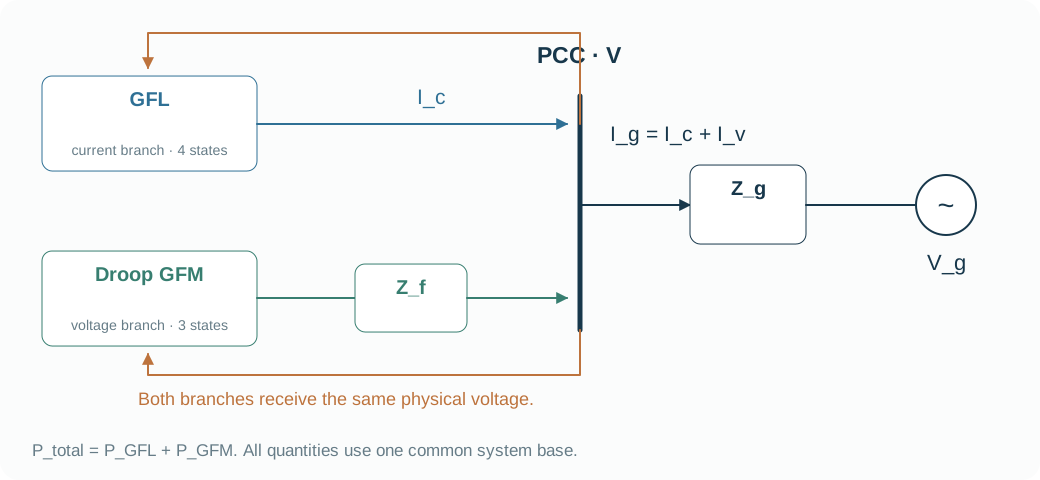
The GFL branch supplies I_c; the GFM branch supplies U behind Z_f. KCL gives I_g = I_c + (U − V)/Z_f. Combining it with V = V_g + Z_gI_g yields one explicit PCC voltage.
Evaluate this voltage first, then express it in each controller’s local frame and compute feedback. The seven states are the four GFL states plus three droop states, but concatenating state vectors alone does not connect the models. The common network does.
I_g=I_c+\frac{U-V}{Z_f},\qquad V=V_g+Z_gI_gV=\frac{V_g+Z_g I_c+(Z_g/Z_f)U}{1+Z_g/Z_f}07.03 MECHANISM & DERIVATION
Distinguish the sharing policy from actual sharing
Compute S_c = VI_c* and S_v = VI_v* at the same PCC. Their instantaneous sum must equal total complex power. Equal command increments do not require equal transient outputs because angle and current dynamics differ.
Inspect branch and total power as SCR decreases. This is a shared-PCC current-source/voltage-source teaching model. The source REGFM_C1 notebook distinguishes an A11 positive-sequence formulation from an F21 detailed research lift; reproducing either requires its own equations and parameters.
S_{PCC}=V(I_c+I_v)^*=S_c+S_vFROM EQUATION TO JUDGMENT
Work the case
On the common 10 kVA base, split a total +0.03 pu power-command increment equally between two branches.
- Total physical increment is 0.03 × 10 kVA = 300 W.
- Each branch receives 150 W.
- On the common base, 150/10000 = 0.015 pu.
Each command increment is 0.015 pu on the common base. That does not assert equal instantaneous branch responses.
FROM PREDICTION TO EVIDENCE
The branches interact before their powers add
An equally split command creates distinct branch trajectories at the common PCC. Their sum follows total power at every sample. The figure shows changes from each initial power to make the small branch transients visible; the lab below displays actual powers.
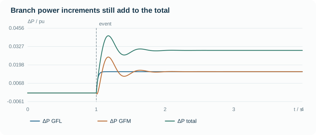
- Each branch command rises by 0.015 pu on the same system base.
- The branch paths differ because PLL/current and droop/angle dynamics interact through V.
- At every sample, the two branch powers sum to the total PCC power.
Your experiment
- Select branch power and compare the two contributions during the +0.03 pu total step.
- Check that the branch powers sum to the total at the event and at the final time.
- Reduce SCR to 2, rerun, and describe which branch response changes more.
Laboratory · Python runs in your browser
Predict → run → inspect
Predict the response, then change a parameter and run. The initial plot is a baseline generated by the same solver. The first computation downloads Python; later runs reuse it.
Loading the baseline…
Numerical audit and samples
Low-frequency teaching realization: nominal-frequency algebraic network and ideal current/voltage realization. 50 Hz, 10 kVA, 400 V; initial PCC total P = 0.6, Q = 0; X/R = 10. τᵢ = 0.02 s, τₚ = 0.1 s, τq = 0.05 s, nq = 0.0325; GFM source impedance 0.00625 + j0.1 pu. LCL, inner PI, DC dynamics and current limits are omitted.
CHECK YOUR REASONING
Can you explain it—and calculate it?
Your engineering decision
Show that branch powers sum to total power at every sample. Then explain one unequal transient interval through the common PCC feedback and the different synchronization mechanisms.
REPRODUCE & EXTEND
Take the evidence into your model
Core equation reference
I_g=I_c+\frac{U-V}{Z_f},\qquad V=V_g+Z_gI_gV=\frac{V_g+Z_g I_c+(Z_g/Z_f)U}{1+Z_g/Z_f}S_{PCC}=V(I_c+I_v)^*=S_c+S_vOpen the Python experiment and model source
The code reads the lab parameters and draws its own result. Edit the experiment or source to test your prediction. Download a single .py file with parameters, solver and experiment; local execution requires Python 3.
case is a snapshot of the controls when you press Run. Call solve(case) and assign the final solution to result to plot it.
The first run needs internet access to download Python. Computation stays in your browser; the solver uses only the standard library.
Ready to run.
Output appears here.
Python result
Inspect and edit the model source (advanced)
Source edits affect the next Python experiment; the lab above retains the original teaching equations.
Source materials and model scope
Based on local PINN-IBR materials reviewed on 2026-10-03. The website uses independent teaching realizations; low-frequency models retain nominal-frequency algebraic networks and ideal actuators. Continue into the detailed models below.
Coding/Modeling/Single-IBR-Infinite-Bus/08_REGFM_C1_Hybrid_Infinite_Bus.ipynbResearch-Xirui-Zhang/Coding/xirui_low_frequency/model.py
WHAT FOLLOWS
Parallel hybrid keeps both mechanisms active. Mode-switching hybrid instead changes the active equations, making state meaning and transition policy decisive.